Repo: Text Sentimental Classification Based on the Twitter Dataset
Introduction
This experiment aims to perform a four-way classification of text using a Twitter sentiment analysis dataset. Text data undergo a series of preprocessing steps to ensure optimal results. We trained five different models, including Decision Trees, Random Forest, Multilayer Perceptron (MLP), Residual Network (ResNet), and a BERT model with a classifier. These models were compared based on their performance on a validation set, with the BERT model chosen as the best due to its superior accuracy. The experiment ultimately showcased the performance of each model on the test set, with the BERT model with a classifier performing best in terms of accuracy.
Data Processing
Dataset
The dataset used in this experiment is a Twitter sentiment analysis dataset. Given a piece of text and an entity, our task is to judge the sentiment of the text towards the entity. This dataset includes four categories: Positive, Negative, Neutral, and Irrelevant. We extract features from the text for subsequent classification. The dataset is large enough to train a variety of models and ensure the models’ generalizability. Each sentiment category is relatively balanced, avoiding the class imbalance issue that could bias the prediction model towards the majority class.
Data Preprocessing
To prepare the data for text analysis, we performed several preprocessing steps:
- Filtering: Filtering out non-alphanumeric characters to clean the data. These characters typically carry little meaning for sentiment analysis tasks and might interfere with the learning process.
- Lowercasing: Converting all text to lowercase to avoid analysis complications and reduce duplicate features since text data is case-sensitive.
Tokenization
Since machine learning models cannot directly understand raw text data, tokenization is the first step in converting text into a numerical form. In this experiment, we used the nltk.word_tokenize module to split the cleaned text into individual word tokens.
Removing Stop Words
Stop words are common words (e.g., “is”, “the”, “and”) that usually don’t carry significant meaning and can be removed to reduce the dimensionality of the feature space. After tokenization, we used nltk.corpus.stopwords to identify and filter out these stop words.
Feature Extraction
We manually implemented Word count feature extraction in this experiment. This method extracts each text into a vector, where the vector’s dimensions are the number of all tokens, and each dimension’s value corresponds to the count of the respective token in the text. Thus, this method results in a high-dimensional, sparse matrix, giving more weight to frequently occurring words.
However, for feature extraction used in subsequent model training, we adopted the Term Frequency-Inverse Document Frequency (TF-IDF) method. It considers not only the frequency of a word in a single document (Term Frequency) but also the inverse of the frequency at which the word appears across all documents (Inverse Document Frequency). This helps to balance the weight given to each word, assigning less weight to words that appear frequently across all documents and more weight to words that appear in specific documents only.
Dimensionality Reduction
For large text corpora, the TF-IDF process generates a high-dimensional feature space. In this experiment, the dimensionality produced by TF-IDF was 30,962. Although higher-dimensional vectors retain more information, they increase computational complexity and can lead to model overfitting. In practical training, we found that recommended dimensionality reduction techniques (e.g., hashing, random projection) might lose significant information. Therefore, we used Truncated Singular Value Decomposition (Truncated SVD) for dimensionality reduction in this experiment. Truncated SVD works directly on the data matrix, unlike PCA, which operates on the covariance matrix, making it more suitable for sparse matrices. After dimensionality reduction with Truncated SVD, the final feature dimensionality was reduced to 100.
Model Implementation
In this experiment, we utilized five different classifiers: Decision Tree (DT), Random Forest (RF), Multilayer Perceptron (MLPClassifier), Text-based Residual Network (TextResNetClassifier), and a Bert model with a classifier (BertClassifier). Decision Tree and Random Forest are directly employed from sklearn’s modules for classification. MLPClassifier, TextResNetClassifier, and BertClassifier, on the other hand, were specifically designed. Decision Tree (DT), Random Forest (RF), MLPClassifier, and TextResNetClassifier were trained on previously extracted features, while BertClassifier used the Bert pre-trained model for word embedding and was then trained with a classifier attached
MLPClassifier
The MLPClassifier is implemented in the ManualModel class, following the sklearn-style interface, and is built using the PyTorch framework. This model consists of an input layer, several hidden layers, and an output layer, with all layers being fully connected. The hidden layers utilize the ReLU activation function. The model employs the Adam optimizer and cross-entropy loss function for training and incorporates techniques like learning rate decay and weight decay for optimization.
BertClassifier
The BertClassifier leverages the pre-trained BERT model from Hugging Face’s transformers library for text classification tasks. This model builds upon the BERT architecture by extracting embedding from input text using the pre-trained BERT model, followed by a dropout layer for regularization and a fully connected layer for classification. The output from the BERT model’s pooler is passed through the dropout and fully connected layer to obtain the final classification results. The model is trained using cross-entropy loss.
TextResNetClassifier
The TextResNetClassifier is a text classification model based on convolutional neural networks. Inspired by the ResNet architecture, it utilizes residual connections to allow gradients to flow directly through the network. The architecture consists of one initial convolutional layer, eight residual blocks, one attention pooling layer, and a final fully connected layer for classification. Each residual block comprises two convolutional layers with batch normalization and dropout. The attention pooling layer in the TextResNetClassifier applies a learned attention mechanism to focus on the most significant parts of the text representation. The final classification is done using a fully connected layer.
Summary
In summary, the MLPClassifier is a straightforward yet effective baseline model. The BertClassifier leverages transfer learning from the pre-trained BERT model, while the TextResNetClassifier introduces convolutional and residual structures to text classification tasks. Designing these different models allows for a comprehensive comparison of various neural network architectures in text classification tasks.
Parameter Tuning
Model hyperparameters were adjusted through a series of trial and error experiments to optimize model performance on the validation set.
BertClassifier
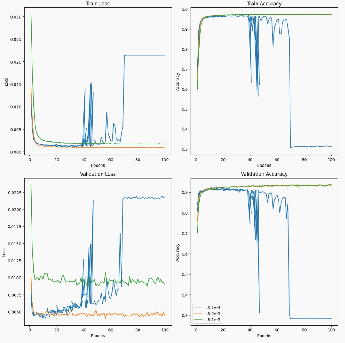
In the case of Bert, different learning rates significantly impact training outcomes. Training results with different learning rates are shown in the figure below. A too high learning rate can cause the model to overshoot the minimum of the loss function, leading to diverging rather than converging loss values. This is why the loss value initially decreases rapidly (due to the high learning rate and large steps) and then rises to a plateau. Conversely, with a too low learning rate, the training process may fail to converge.
TextResNetClassifier
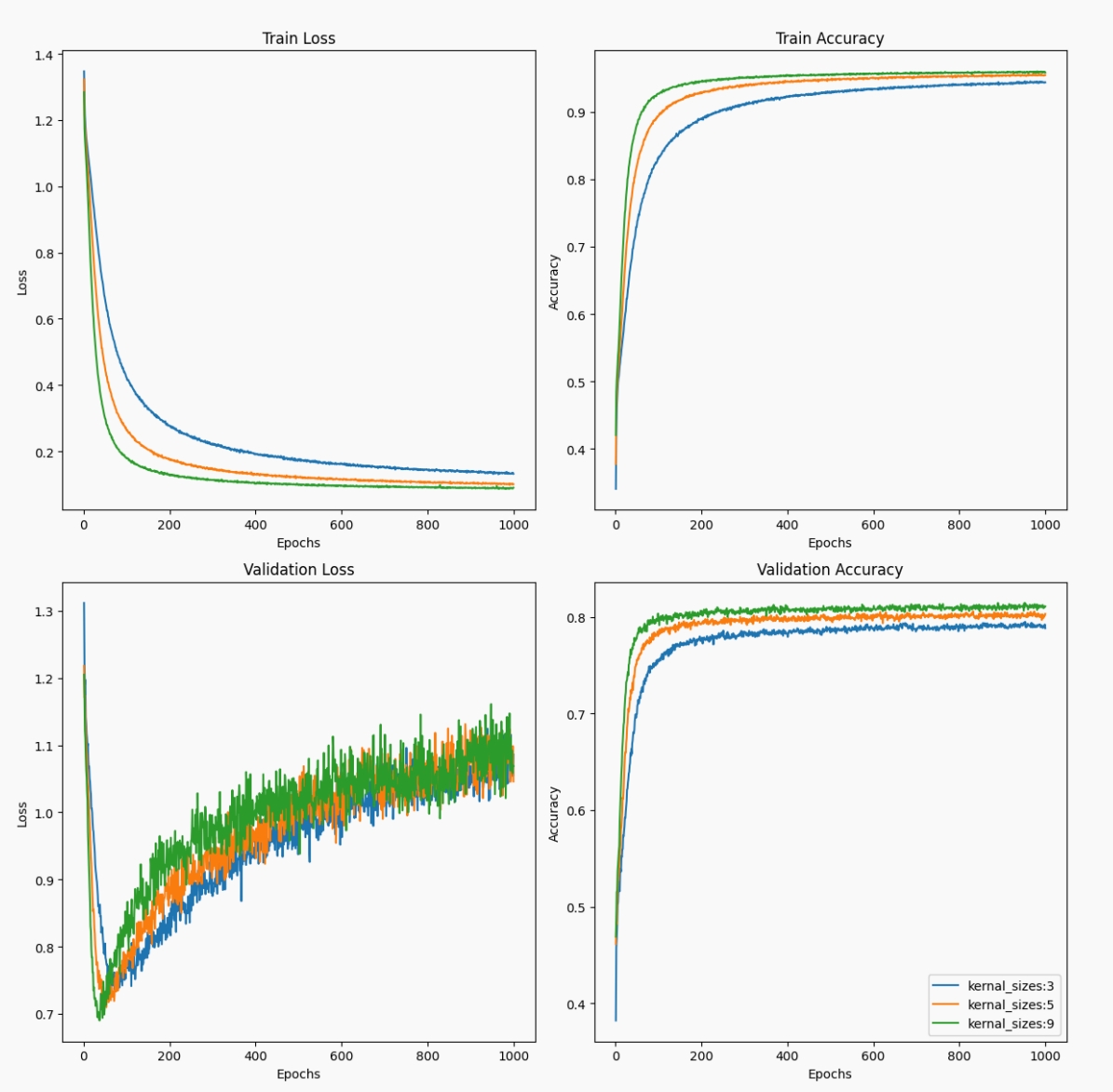
Due to batch normalization technology, adjustments in learning rate did not significantly affect TextResNet’s final outcome during parameter tuning. However, unlike image classification, we found that using larger convolutional kernels yielded better results, as shown in the figure below. For text data, larger convolutional kernels can capture more contextual information in a single convolution operation. Thus, long-range contextual information may be more helpful for text classification tasks. Additionally, text data typically has lower dimensions than image data, allowing for the use of larger convolutional kernels without a drastic increase in the number of parameters.
Performance and Computational Efficiency
The table below shows the computational efficiency and performance of the three models, all trained on an NVIDIA A100 80GB PCIe:
| Model | Time/Epoch | Total Training Time | GPU Memory Usage (MiB) | Hyperparameters |
|---|---|---|---|---|
| BertClassifier | 3 minutes | 4 hours | 5641 | Max token length: 64, Batch size: 64, Epochs: 75, Learning rate: 2e-5, Dropout: 0.1 |
| TextResNetClassifier | 30 seconds | 7-8 hours | 1881 | Batch size: 32, Learning rate: 0.001, Epochs: 890, Dropout: 0.5, Kernel size |